A general proposal for choosing the number of imputations

From chapter 14 of the multiple imputation book

This September marked the release of a book of singular magnificence: Multiple Imputation and its Application by James Carpenter, Jonathan Bartlett¹, myself, Angela Wood, Matteo Quartagno, and Mike Kenward.

I was responsible for drafting most of chapter 14, ‘Using multiple imputation in practice’, which covers how to approach analysis with missing data, considering whether you need multiple imputation, choosing the number of imputations, using random number seeds, and reporting of analyses after multiple imputation.

On the topic of choosing the number of imputations, I started by looking at two methods:

1. The ‘linear rule’ proposed by Bodner², then justified and popularised by White, Royston & Wood³.

2. A two-stage method proposed by von Hippel⁴.

Essentially the linear rule says that you need as many imputations as incomplete cases. This controls the Monte Carlo standard error (MCSE; see the White, Royston & Wood paper) of a multiple imputation point estimator to be less than 10% of its estimated SE.

The von Hippel method aims to control the MCSE of the SE estimator⁵, and does this through the fraction of missing information (FMI: the statistical information missing about a parameter compared with the information we would have without missing data). Since the fraction of missing information is unknown, we have to estimate it. How do we do that? We produce an initial number of imputations, estimate FMI, and plug-in the estimate (or an upper confidence limit) to his formula. This two-stage approach adds a layer of complexity that the linear rule doesn’t have.

When thinking about the two-stage approach, it seemed like there might be a more direct method. I’ve done a lot of thinking about Monte Carlo error in the context of simulation studies. There, when we don’t know how many repetitions we’ll need, we sometimes produce an initial number (say 500), estimate the MCSE, and use that to decide how many more would reduce MCSE to an acceptable level (e.g. I did this for our letter on not fixing the complete data⁶ and was happy with MCSE after the initial 500 reps). The way we pick how many more reps we need is to note that MCSE is a function of

\(\sqrt{\frac{1}{n_{reps}}}.\)

We plug-in the estimated MCSE (noting that ideally we would use the true MCSE given n_reps) and solve for the number of reps required. By analogy, the MCSE of a multiple imputation statistic is a function of

\(\sqrt\frac{1}{\text{number of imputations}}.\)

So why not take the same approach as in simulation studies? The nice thing about it is that you can work on any statistic estimated by MI. The linear rule targets the MCSE of a point estimator; the von Hippel approach targets the MCSE of a standard error estimator; my proposal can target any statistic (for most statistics other than point estimate, the MCSE is estimated using jackknife in Stata’s ‘mi estimate, mcerror’ and Alessandro Gasparini implemented the same in mice.mcerror).

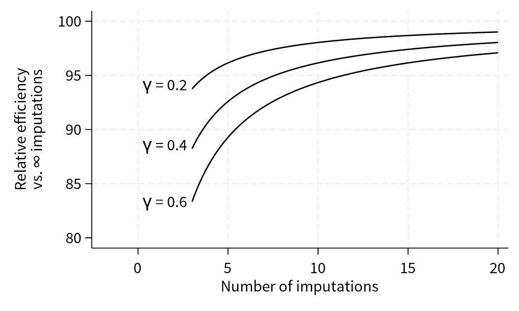
I wrote down the idea and had a chat with James Carpenter. He liked it and said to stick it into chapter 14 but note that it was a proposal and hadn’t been evaluated (I’d call it phase I⁷). I’m think it’s worth doing some simulation work to check that it does control MCSE to the required level. I’d guess it’s slightly conservative for some statistics. Suppose you want the MCSE of a standard error, or a confidence bound. Then we know that multiple imputation becomes more efficient as you increase the number of imputations (see the figure below, note that γ is the true FMI, see footnote for Stata code⁸). That means that the standard error or the confidence bound will be changing as the number of imputations increases.

Anyway, I’m now collaborating with a couple of people on evaluation of this proposal and finding it super interesting. Interestingly, the person leading it has thought of a way to reduce the error due to plugging in an estimate of the MCSE after an initial number of imputations. One of those ‘obvious once you’ve said it’ things.

1. Jonathan recently posted about it on his blog (if you don’t already read Jonathan’s blog, it’s superb and where a lot of statisticians go to learn and understand things)

2. TE Bodner. What Improves with Increased Missing Data Imputations? Structural Equation Modeling, 2008; 15(4): 651–675. https://doi.org/10.1080/10705510802339072

3. IR White, P Royston and AM Wood. Multiple imputation using chained equations: issues and guidance for practice. Statistics in Medicine, 2011; 30(4): 377–399. https://doi.org/10.1002/sim.4067

4. PT von Hippel. How many imputations do you need? A two-stage calculation using a quadratic rule. Sociological Methods & Research, 2020; 49(3): 699–718. https://doi.org/10.1177/0049124117747303

5. Interestingly von Hippel’s paper never explicitly uses the term Monte Carlo SE and denotes is as the SD of an estimated SE. It’s intentional because the short Stata program he provided does use things named MC.

6. TP Morris, IR White, S Cro, JW Bartlett, JR Carpenter and TM Pham. Comment on Oberman & Vink: Should we fix or simulate the complete data in simulation studies evaluating missing data methods? Biometrical Journal. 2023. https://doi.org/10.1002/bimj.202300085

7. G Heinze, A-L Boulesteix, M Kammer, TP Morris and IR White for the Simulation Panel of the sᴛʀᴀᴛᴏs initiative. Phases of methodological research in biostatistics—Building the evidence base for new methods. Biometrical Journal, 2023. https://doi.org/10.1002/bimj.202200222

8

* Stata code for figure
#delimit ;
twoway
    (function (100/(1+(.2/x))), range(3 20) lc(black))
    (function (100/(1+(.4/x))), range(3 20) lc(black))
    (function (100/(1+(.6/x))), range(3 20) lc(black))
    ,
    ytitle("Relative efficiency" "vs. {&infin} imputations")
    xtitle("Number of imputations")
    xscale(range(-2 20))
    legend(off) scale(*1.5)
    text(`=100/(1+(.2/3.2))' 1.5 "{&gamma} = 0.2")
    text(`=100/(1+(.4/3.1))' 1.5 "{&gamma} = 0.4")
    text(`=100/(1+(.6/3))' 1.5 "{&gamma} = 0.6")
    ;
#delimit cr